Nickname Generation with Recurrent Neural Networks with PyTorch

John Walk

August 2020

This was originally published on the Pluralsight tech blog.

Anyone who’s attended one of the PAX gaming conventions has encountered a group called (somewhat tongue-in-cheek) the “Enforcers”. This community-driven group handles much of the operations of the convention, including anything from organizing queues for activities (and entertaining people in them) to managing libraries of games or consoles for checkout. Traditionally, Enforcers will often use an old-school forum handle during the convention, with the pragmatic outcome of easily distinguishing between Enforcers with common names, but also bringing some personal style – some even prefer to be addressed by handle over their real name during a PAX. Handles like Waterbeards, Gundabad, Durinthal, bluebombardier, Dandelion, ETSD, Avogabro, or IaMaTrEe will draw variously from ordinary names, puns, personal background, or literary/pop-culture references.

At PAX East this past February, we hit upon the idea of building a model to generate new Enforcer handles. This a perfect use case for a sequential model, like a recurrent neural network – by training on a sequence of data, the model learns to generate new sequences for a given seed (in this case, predicting each successive character based on the word so far).

Our goal here is twofold:

• to explore building a recurrent neural network in PyTorch (which is new ground for me, as most of our production implementations are in Tensorflow instead)
• to demonstrate the power of transfer learning.

Let’s dive in!

Recurrent Neural Networks for sequence modeling

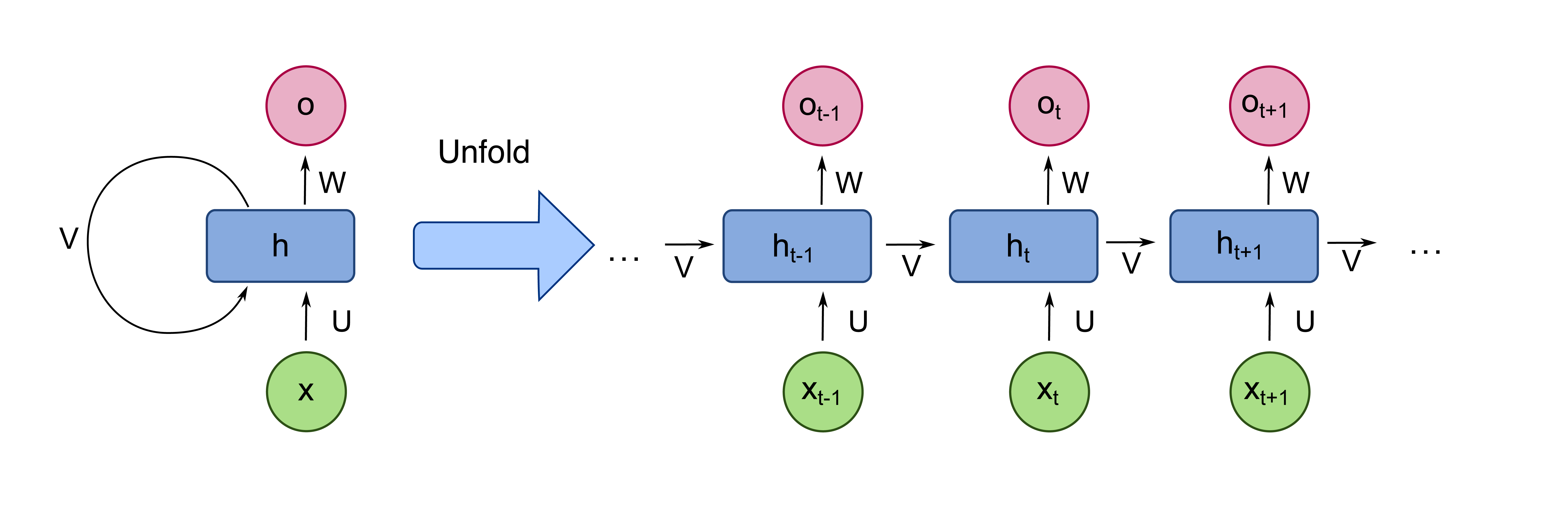
When modeling sequential data (audio, natural-language text, etc.) we need to carefully consider our architecture – the temporal interaction between each point in the sequence is frequently significantly more important as the content at any given single point. We therefore need a way to assemble and encode the sequence’s interactions, and combine this with the input at each point in the sequence to generate a meaningful output. Recurrent neural networks (RNNs) achieve this by encoding a sequence-dependent “hidden state” in the network – at each time step, the network takes both its input for that step and the hidden state from the previous step, and uses that to generate both the time step’s output and an updated hidden state passed to the next step, visualized below:

© Wikimedia Commons User:fdeloche / CC-BY-SA-4.0

This architecture can handle mapping single or multiple values at the input and/or the output, i.e., we can do many-to-one, many-to-many, or one-to-many processing tasks. For example, we might care about a many-to-one mapping for sequence classification, inputting a sequence of inputs and generating a single output label. Where RNNs are particularly applicable, though, is the many-to-many task (also called sequence-to-sequence), inputting a series of inputs and generating a new, different sequence (for example, inputting a sentence of English text to Google Translate and getting a French sentence out).

In principle, the network’s operation on the hidden state can be simple – take, for example, the linear combination of the input and hidden-state vector and typical nonlinear activation (e.g., a sigmoid function) found in early Elman networks. However, as this essentially equivalent to constructing an extremely deep feed-forward network (with layers multiplied out per timestep), this is subject to the “vanishing gradient” problem, where the network gets stuck in an untrainable state as parameter updates get progressively weaker as smaller gradients of the loss with regard to the weights are compounded by chaining through many layers of the network. In a recurrent network, this has the effect of the network “losing information” over sufficiently long sequences.

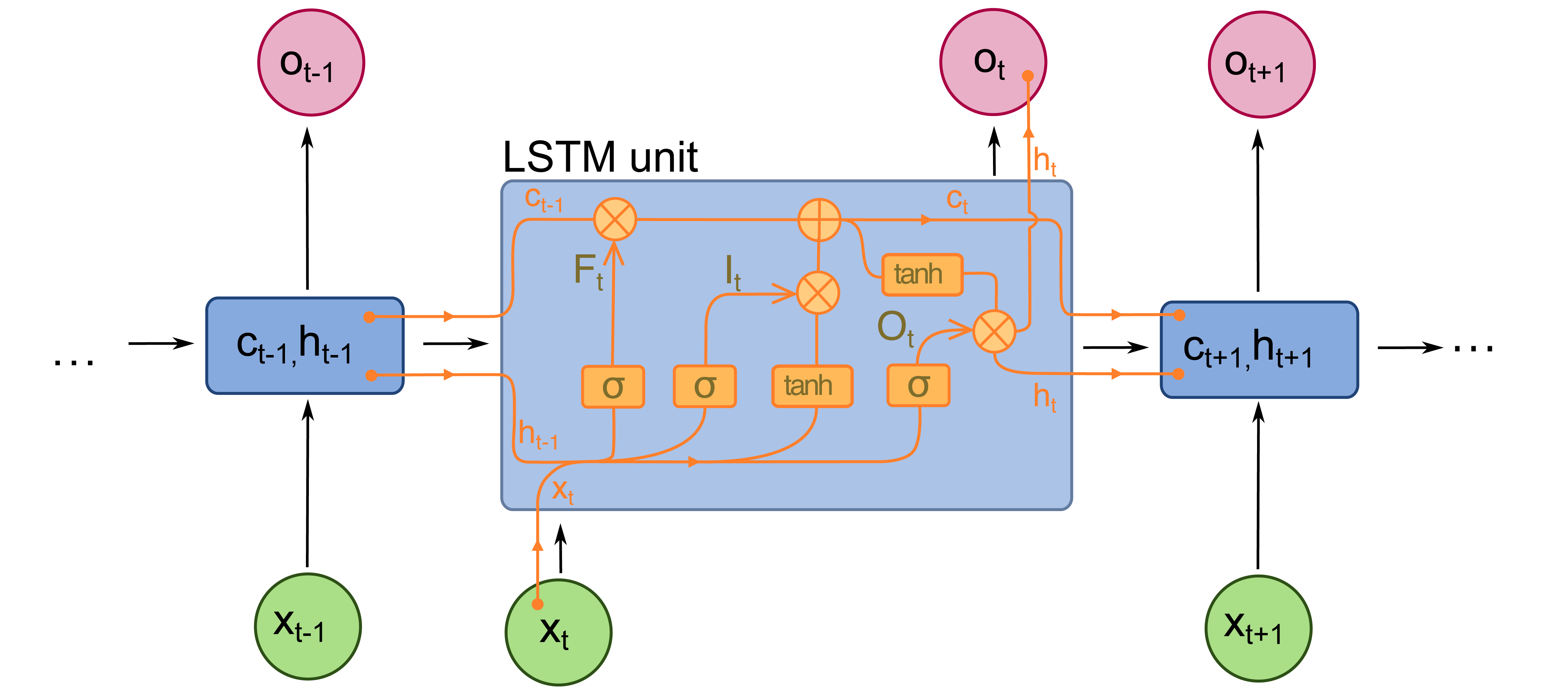
As such, much of the more recent research in deep learning on sequences has focused on retaining information over long sequences. For example, Long Short-Term Memory (LSTM, illustrated below) or Gated Recurrent Unit (GRU) networks include separate learnable parameters specifically for retaining or forgetting information over long sequences, rather than blindly squashing parameters through gradient updates over every point of the sequence.

© Wikimedia Commons User:fdeloche / CC-BY-SA-4.0

More recently, research has particularly focused on attention mechanisms for sequence-to-sequence models – the attention layer learns for each point in a sequence to give boosted or suppressed weight to other steps in the sequence, without dependence on the in-between (whereas a recurrent mechanism inherently must step through every intervening point to compute its state). This essentially learns to pay particular attention (whence the name) to certain other points regardless of their proximity in the sequence, enhancing the network’s ability to retain information over long sequences. While attention can be used in combination with recurrent operations, recent research has culminated in the Transformer architecture, which dispenses with recurrence entirely and relies solely on attention mechanisms. Transformer-based language models like BERT or GPT-2 (and now GPT-3) are currently state-of-the-art for a number of language modeling tasks.

As we’re working with relatively short sequences for this task, we realistically don’t have to be too fussed with retaining long-term information over our sequences. However, PyTorch includes cookiecutter approaches to building more complex components like LSTMs or GRUs, so we’re not really losing anything by using a more modern approach – we’ll use an LSTM layer for this project.

what do we do when we’re short on data?

In modern deep learning, potential model complexity can easily outpace the scale of the data you have to train it on. For example, the InceptionV3 computer-vision architecture, with approximately 23 million tuneable parameters, doesn’t necessarily help you if you only have a few thousand images to train on. Even worse, the GPT-2 natural-language model, with some 1.5 billion parameters, not only requires learning on an utterly massive text corpus, its training is so computationally expensive that it has a significant carbon footprint. Fortunately, there are several techniques to utilize larger separate datasets and/or previous computation to bootstrap complex models from relatively limited data – here, we’ll consider pretraining and transfer learning.

In both of these cases, we’re reusing previous computation on other data: for a given model architecture, rather than training the model from scratch with randomly-initialized weights, we instantiate some or all of the model with weights that have been previously trained. We can then use these weights either as a “warm” starting point for fine-tuning, or simply use them as-is, essentially as a fixed function converting our inputs into some learned representation. By doing so, we reduce a large model architecture effectively into a smaller model more suited for our data size and time constraints.

With simple pretraining, we’re expecting essentially the same data as inputs. For example, we might use pretrained unsupervised word embeddings as the input to a larger language model, but in that case we’re just using the word-level embeddings as-is to convert our text to a dense vector representation. Effectively, we’re assuming the inputs used in pretraining are from roughly the same distribution as our data of interest. (In some cases, it may literally be the same distribution – “warm start” training for models is useful to continuously update a live model as more data comes into an ML-powered system over time.)

Where these techniques really shine, though is in transfer learning – that is, we use a model trained on a fundamentally different dataset than our actual use case, aiming to exploit underlying similarities between the datasets. I find this easiest to visualize in the case of computer-vision models (though it’s applicable in many other instances!). In a deep convolutional neural network, the earliest layers are learning relatively simple filters (recognizing things like light vs. dark, or sharp edges) that would be common in essentially any image. So, rather than trying to train from scratch on a small, specialized dataset, we can utilize deep architectures trained on massive datasets like ImageNet for generalizable early layers of the model, and only need to worry about training the last few layers for our particular task. So, we could (for example) use a state-of-the-art architecture despite a small dataset (for, say, binary “hotdog vs. not-hotdog” classification) – even if that label set is not in the original, shared training data at all!

In the case of our handle generator, this will be absolutely necessary, as we only have a handful of existing Enforcer handles to work with. However, most of the task for our RNN will simply be figuring out which character combinations are vaguely sensical as phonemes (which can be a tall order, since English orthography is a bit of a trash fire), so there’s nothing stopping us from using other English text (or even other human names) to handle most of the training!

data prep

For our work here, we’ll work with three data sources:

• the full text of Frankenstein; or, The Modern Prometheus by Mary Wollstonecraft Shelley (available in the public domain here from Project Gutenberg).
• a set of real names generated by Faker, which emits permutations of common first and last names, with randomized suffixes.
• our Enforcer handle dataset (collected by opt-in from the community, and somewhat obfuscated in this article for privacy reasons).

We’ll use the general text and real-name datasets to tune our model to generate plausible combinations for pronounceable phonemes and name-like structures, before fine-tuning on Enforcer handles. For consistency, we’ll enforce some transformations (like allowing hyphenated or cap-cased words) but otherwise shouldn’t need much preprocessing.

text representation

First, we need to represent our text inputs numerically – for a word-level model, this would entail stopword treatment, potentially stemming or lemmatizing words, tokenizing and vectorizing a large (potentially millions of unique tokens) vocabulary, which can be fairly complex and computationally expensive in its own right. Fortunately, representing a character-level dataset is much simpler - we simply need to represent each lower and upper case ASCII letter, plus a hyphen and apostrophe (since we want to retain these for our generator), which we can do from scratch in lookup dictionaries:

LETTERS = string.ascii_letters + "-'"
charset_size = len(LETTERS) + 1  # add one for an EOS character
char_index = {char: i for i, char in enumerate(LETTERS)}
inverse_index = {i: char for char, i in char_index.items()}
inverse_index[charset_size - 1] = "<EOS>"

which builds up an ordinal index of each character, plus its inverse (where we also include an end-of-sequence character, which won’t be present in our input data but can be produced by the generator).

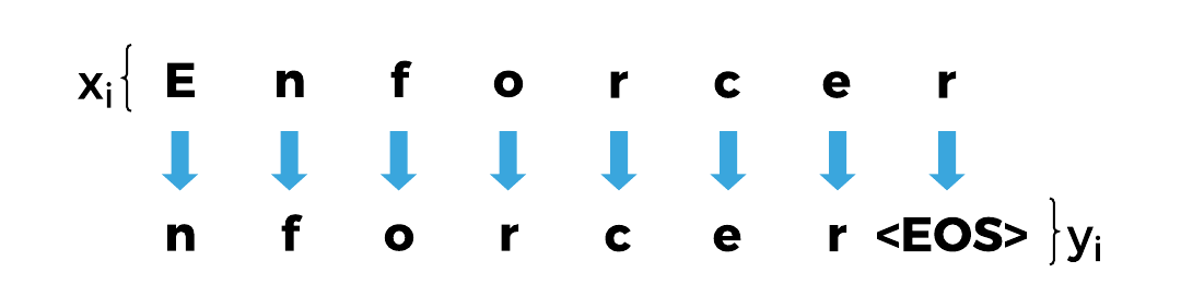
Next, we need to use these indices to represent the text as PyTorch Tensors. Specifically we need tensors that, at each step of the sequence, encode the numeric index of the character as input, and the index of the next character in the sequence (including an explicit end-of-sequence marker) as the output – we’ll then train the network to successively predict the next character in the sequence at each time step.

We’ll use a tensorize function to build these for an input text. We could use this input tensor to generate a one-hot encoding (i.e., a binary vector indicating with the nonzero index which character is represented), but for now we’ll lay out our network architecture such that we only need the integer indices of each character for both the input and the output.

TensorPair = typing.Tuple[torch.LongTensor, torch.LongTensor]

def tensorize(word: str) -> TensorPair:
    input_tensor = torch.LongTensor([char_index[char] for char in word])

    eos = torch.zeros(1).type(torch.LongTensor) + (charset_size - 1)
    target_tensor = torch.cat((letter_indices[1:], eos))

    return input_tensor, target_tensor

data management in PyTorch

To manage our inputs, we’ll use PyTorch’s built-in data managers – the Dataset and DataLoader classes. The Dataset class gives us a useful wrapper to manage data loading and preprocessing – we simply need to either supply a way to access the data as an underlying iterable (“iterable-style”) or by defining indexed lookup across a known scope of data (“map-style”).

For example, we can represent our Frankenstein dataset as below:

class FrankenDataset(torch.utils.data.Dataset):
    def __init__(self, path_to_text: str):
        with open(path_to_text, "r") as rf:
            text = rf.read()
            text = text.replace("\n", " ").strip()  # compress newlines
            text = re.sub(r"[^a-zA-Z\-' ", "", text)  # strip undesired characters
            text = re.sub(r" {2,}", " ", text)  # compress whitespace runs to single space
            self.words = text.split(" ")

    def __len__(self) -> int:
        return len(self.words)

    def __getitem__(self, idx: int) -> TensorPair:
        return tensorize(self.words[idx])

Here we handle all the string cleaning on dataset initialization, and need only provide the __len__ and __getitem__ methods to support map-style access. This class loads all of its data into memory – this isn’t an issue for such a small dataset (~75k tokens, for Frankenstein) but won’t work for very large datasets. However, with some cleverness and disk-caching, we could (for example) use the __getitem__ method to instead lazily load data from disk, and only need to store a list of reference locations.

Once we have a Dataset defined, we can pass that through a DataLoader to manage data shuffling and batching (trivial here, as we’re using single-sample minibatches to simplify working with variable-length sequences):

frank = FrankenDataset(path_to_text)
franken_loader = torch.utils.data.DataLoader(
    frank,
    batch_size=1,
    shuffle=True
)

To feed data into our model, we simply loop over the franken_loader object, which will yield shuffled, randomized batches (single samples, in our case) on each iteration. (Users should note that the DataLoader will add a batch dimension to the front of the tensors emitted by the Dataset, of length batch_size.)

Map-style datasets like we used in FrankenDataset require us to know the entire scope of the dataset, and be able to directly access samples by index (which the DataLoader then uses to generate randomized batches). In some cases, though, it may be simpler to simply directly support iteration on the data itself (for example, when consuming data from a streaming system). For these use-cases, newer (version 1.2+) PyTorch supports an IterableDataset type, which simply needs an __iter__ method returning a Python iterable to be defined – the DataLoader then will simply access this iterator in-order rather than constructing batches by randomly-selected index.

For our Faker-generated real names, we already have a good degree of randomization in our data, so this should be straightforward. We can even generate names from multiple national localizations, though we’ll need to take some care to ensure that we’re complying with our chosen character set – this means folding unicode characters to their ASCII equivalents, and skipping providers that aren’t easily ASCII-translatable (though Faker itself has no trouble providing non-Latin-alphabet data!). In this case, we’ll sprinkle Finnish, Spanish, German, and Norwegian names into the mix, along with our common English names. We can generate these names, clean ASCII characters and enforce minimum length, and randomly transform them to be hyphenated or CapCased (as either can appear in our Enforcer handles) before emitting them in a generator returned by the __iter__ method, as below:

class FakerNameDataset(torch.utils.data.IterableDataset):
    def __init__(self, n_samples=5000):
        self.n_samples = n_samples
        self.namegen = faker.Faker(  # draw from multiple language providers
            OrderedDict([
                ("en", 5),
                ("fi_FI", 1),
                ("es_ES", 1),
                ("de_DE", 1),
                ("no_NO", 1)
            ])
        )

    def __iter__(self) -> Iterable[TensorPair]:
        return (tensorizer(self.generate_name()) for _ in range(self.n_samples))

    def generate_name(self) -> str:
        name = self.namegen.name()

        # fold unicode characters to nearest ascii
        name = "".join(
            char for char in unicodedata.normalize("NFKD", name)
            if not unicodedata.combining(char)
        )
        # clean further characters
        name = re.sub("[^a-zA-Z\-' ]", "", name)

        # randomly map to hyphenated or CapCased
        if random.uniform(0, 1) < 0.5:
            return name.replace(" ", "")
        else:
            return name.replace(" ", "-")

This works out of the box with PyTorch’s DataLoader, and we don’t even need to set the batching or shuffle parameters!

names = FakerNameDataset(n_samples=30000)
name_loader = torch.utils.data.DataLoader(names)

Finally, our Enforcer dataset is straightforward, as the handles are already formatted nicely, so that’ll be structured into an EnforcerHandleDataset identically to the FrankenDataset.

building our network

We could, in principle, build our RNN using only PyTorch tensor operations (after all, neural networks are just large piles of linear algebra) and activation functions – but this is tedious and excessively difficult for complex components (like the LSTM). Instead, we’ll use PyTorch’s straightforward building blocks to define our network.

For this, we define our RNN as a subclass of torch.nn.Module, which encapsulates the structure of the network and its operations, and comes out of the box with all the setup needed for state tracking, gradient computation, etc. We simply need to define the components in the network (which are themselves Module subclasses) as attributes in __init__, and a forward method that lays out the computation for a “forward pass” (input-to-prediction) of data flowing through the network.

class CharLSTM(torch.nn.Module):
    def __init__(
        self,
        charset_size: int,
        hidden_size: int,
        embedding_dim: int = 8,
        num_layers: int = 2
    ):
        super(CharLSTM, self).__init__()

        self.charset_size = charset_size
        self.hidden_size = hidden_size
        self.embedding_dim = embedding_dim
        self.num_layers = num_layers

        self.embedding = torch.nn.Embedding(charset_size, embedding_dim)
        self.lstm = torch.nn.LSTM(
            embedding_dim,
            hidden_size,
            batch_first=True,
            num_layers=num_layers,
            dropout=0.5
        )
        self.decoder = torch.nn.Linear(hidden_size, charset_size)
        self.dropout = torch.nn.Dropout(p=0.25)
        self.softmax = torch.nn.LogSoftmax(dim=2)

    def forward(self, input_tensor, hidden_state):
        embedded = self.embedding(input_tensor)
        output, hidden_state = self.lstm(input_tensor, hidden_state)
        output = self.decoder(output)
        output = self.dropout(output)
        output = self.softmax(output)
        return output, hidden_state

    def init_hidden(self):
        return (
            torch.zeros(self.num_layers, 1, self.hidden_size),
            torch.zeros(self.num_layers, 1, self.hidden_size)
        )

This is fairly dense, so let’s step through the components one by one in the forward pass:

1. We pass in the input_tensor generated by tensorize() and our DataLoader. This is a tensor of integers of size (batch_len, sequence_len) representing the character indices. (Remember that we’re using single-sample minibatches here, so batch_len = 1.)

2. An embedding layer grabs an embedding_dim-sized dense vector based on the index of each character (which is just a sparse representation of a one-hot vector for each character) in the input. This produces a tensor of floats of size (batch_len, sequence_len, embedding_dim). In principle, we could skip this step, and pass one-hot vectors of size (batch_len, sequence_len, charset_size) directly to the LSTM layer – since our character-set “vocabulary” is small, this is not a horrifically sparse representation (as it would be for word-level representations). In practice, though, reducing the charset vectors to a small embedding vector improves performance, so we may as well keep it. (This also means you can use this same type of network structure as-is for word-level representations, replacing charset_size with the vocabulary size for your tokenizer.)

3. We run this character representation through the LSTM layer – this also requires a set of tensors representing the hidden states and cell states (held in hidden_state and initialized to zeroes by init_hidden()). This tracks the state of the network through each step of the sequence in a single pass, so we don’t need to iterate over the sequence explicitly, and for single-sample batches is perfectly fine handling variable-length sequences. This produces a tensor of size (batch_len, sequence_len, hidden_size) as well as updated hidden-state tensors.

4. A densely-connected linear layer decodes the LSTM output back into our charset, producing a tensor of size (batch_len, sequence_len, charset_size). This tensor also is fed through a dropout layer during training, which will ignore individual connections probabilistically on each training pass.

5. This is run through a LogSoftmax, which converts the last dimension of the tensor to the logarithm of softmax probabilities of each character. Effectively, we’re building the encoder-decoder architecture common in sequence models here – our embedding and LSTM layers encode the input in a learned internal representation, and the linear layer and softmax decodes this back into a representation in our original characters. This produces both the form expected by our negative-log-likelihood cost function, and an interpretable output, as the maximum log-probability value for each step of the sequence indicates its predicted next character.

6. We then return both the output tensor of probabilities of size (batch_len, sequence_len, charset_size) and the updated hidden state, to be used in the next training or inference step.

We initialize the model like a typical Python class, and can see what we’ve built:

rnn = CharLSTM(charset_size, hidden_size=128, embedding_dim=8, num_layers=2)

which produces

>>> print(rnn)
CharLSTM(
  (embedding): Embedding(55, 8)
  (lstm): LSTM(8, 128, num_layers=2, batch_first=True, dropout=0.5)
  (linear): Linear(in_features=128, out_features=55, bias=True)
  (dropout): Dropout(p=0.25, inplace=False)
  (softmax): LogSoftmax()
)

We can draw samples from this by converting a seed text to a tensor, priming the network, and successively generating outputs by inputting the previously generated character:

def sample(
    seed: str,
    max_len: int = 10,
    break_on_eos: bool = True,
    eval_mode: bool = True
) -> str:
    # optionally set evaluation mode to disable dropout
    if eval_mode:
        rnn.eval()

    # disable gradient computation
    with torch.no_grad():
        input_tensor, _ = tensorize(seed)
        hidden = rnn.init_hidden()

        # add the length-1 batch dimension to match output from Dataset
        input_tensor = input_tensor.unsqueeze(0)

        output_name = seed
        for _ in range(max_len):
            output, hidden = rnn(input_tensor, hidden)
            _, topi = output[:, -1, :].topk(1)  # grab top prediction for last character
            next_char = inverse_index[int(topi.squeeze())]

            if break_on_eos and (next_char == "<EOS>"):
                break
            output_name += next_char
            input_tensor = topi

    # ensure training mode is (re-)enabled
    rnn.train()
    return output_name

There are two important traits to notice here, as they’re a somewhat unintuitive aspect of PyTorch’s API: the torch.no_grad() context block, and the setting of rnn.eval()/rnn.train(). The no_grad() context block disables automatic gradient computation, preventing the model from updating its weights during an inference pass as well as freeing up the unneeded memory and computation that would’ve gone into tracking gradients through the network. The train()/eval() setting toggles the model between “training” and “evaluation” mode, which alters the behavior of certain layers during a forward pass – for example, in training mode a dropout call will randomly skip certain weights, while in evaluation mode every weight is used.

This is important in most inference tasks, as without it the predicted output will be of degraded confidence, and fundamentally nondeterministic (since weights as dropped at random), and it is recommended to use both settings during inference. However, we can optionally perform inference here with evaluation mode turned off (thus, dropout turned on) to introduce some stochasticity to our predictions, which should have a similar effect to using temperature in our outputs.

training!

Of course, drawing the samples right now from the network will produce gibberish, as the network is still using its randomly-initialized weights:

for _ in range(10):
    seed = random.choice(string.ascii_lowercase)
    print(f"{seed} --> {sample(seed)}")

resulting in

v --> vllllllllll
d --> dllllllllll
j --> jllllllllll
z --> zllllllllll
f --> fllllllllll
d --> dllllllllll
w --> wllllllllll
e --> ellllllllll
f --> fllllllllll
q --> qllllllllll

We need to train the network on our dataset. In PyTorch, this follows a fairly typical pattern, although it’s significantly more detailed than the high-level abstraction found in something like Keras (where for the most part you’d simply call a fit method), although bare Tensorflow follows a similar structure. In general, each training step will do the following:

1. zero out the gradients stored in the model
2. compute the output from the model for the training input
3. compute the loss for that output versus that training sample, based on a predefined loss function
4. compute the gradients in the model with regard to that loss, via PyTorch’s automatic gradient tracking
5. step an optimizer to update the model weights based on the computed gradients

In code, this looks something like

criterion = torch.nn.NLLLoss()
optimizer = torch.optim.RMSprop(rnn.parameters(), lr=0.0001)

def train_step(
    input_tensor: torch.LongTensor,
    target_tensor: torch.LongTensor
) -> float:
    optimizer.zero_grad()

    hidden = rnn.init_hidden()
    output, hidden = rnn(input_tensor, hidden)
    loss = criterion(output[0, :, :], target_tensor[0, :])

    loss.backward()  # computes gradients w.r.t. and stores gradient values on parameters
    optimizer.step()  # is already aware of the parameters in the model, uses those gradients

    return loss.item()  # grabs value of NLL loss, rather than graph tracking

In which we utilize a negative-log-likelihood loss function (NLLLoss) and an RMSprop optimizer (though we could certainly use one of the other options supplied by torch.optim, like pure stochastic gradient descent or Adam). We pass in batches (single samples, in our case) of data simply by iterating over our DataLoader object of choice:

losses = []
running_loss = 0.0

for epoch in range(n_epochs):
    looper = tqdm.tqdm(franken_loader, desc=f"epoch {epoch + 1}")
    for i, tensors in enumerate(looper):
        loss = train_step(*tensors)
        running_loss += loss
        losses.append(loss)
        if (i+1) % 50 == 0:
            looper.set_postfix({"Loss": running_loss/50.})
            running_loss = 0

Frankenstein pre-training

After two epochs of training, the sampler is already starting to produce sensical results (including converging to some common words):

seed --> output
---------------
c --> could
h --> he
g --> gare
k --> kear
t --> the
p --> prome
e --> ender
v --> ve
a --> a<EOS>

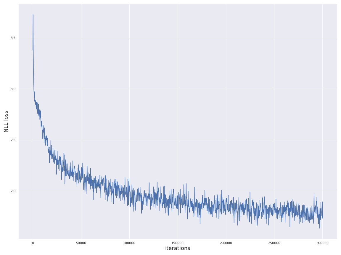
and after a further two epochs, the training loss is largely stabilized:

seed --> output
---------------
n --> not
y --> you
h --> he
e --> ever
q --> quitted
z --> zhe
w --> was
d --> destreated
j --> jound
s --> so
v --> very
p --> part
l --> life
r --> rest
x --> xone

We can see a bit more diversity in results by disabling evaluation mode (which means the dropout layers will still be active during sampling). This should degrade outputs somewhat (since it’s losing connections at random, it should no longer be outputting a best-likelihood estimate of the next character) but is necessary to vary our outputs. In evaluation mode, the output for a given seed is deterministic, so we’d only ever generate one word per seed, and extending to sample a longer sequence is unhelpful as the output will generally die off after producing an EOS character. For our use case, being able to generate a number of candidate words is useful – and frankly, it’ll be cool to introduce a little anarchy to our generated words.

seed --> output
---------------
e --> evil
e --> endeares
e --> expented
e --> endear
e --> eves
e --> earss
e --> eart
e --> exest
e --> enter
e --> endestent
e --> ente
e --> eviled
e --> endeares

At this point, it’s a good idea to save a checkpoint of our model that we can return to as we iterate on later training steps. In PyTorch, we can save the state_dict objects of both our model and optimizer into a single object – provided we can instantiate the same object class, we can then load these to rebuild a snapshot state of the model and training environment. Since this works with general Python object serialization (while conventionally these save files are marked as .pt or .pth, it’s just using pickle under the hood), we can also bundle other training metadata in.

torch.save(
    {
        "model_state_dict": rnn.state_dict(),
        "optimizer_state_dict": optimizer.state_dict(),
        "losses": losses
    },
    pretrain_save_filepath
)

human-name tuning

We’re now ready to start fine-tuning our model. We can easily load our saved checkpoint if we want to start fresh in a new Python session, as below:

rnn = CharLSTM(charset_size, hidden_size=128, embedding_dim=8, num_layers=2)
optimizer = torch.optim.RMSprop(rnn.parameters(), lr=0.0001)

checkpoint = torch.load(pretrain_save_filepath)
rnn.load_state_dict(checkpoint["model_state_dict"])
optimizer.load_state_dict(checkpoint["optimizer_state_dict"])
losses = checkpoint["losses"]

Note that we need to create a fresh instance of the rnn and optimizer objects, and the model needs to be of the same construction as the original – you’ll know it’s gone right if you see an <All keys matched successfully> message when you load the state dictionary for the model instance. With our model loaded, fine-tuning the training is simply a matter of resuming the training loop above, but feeding from the Faker-generated name dataset via name_loader:

running_loss = 0.0

looper = tqdm.tqdm(name_loader, desc="name fine tuning")
for i, tensors in enumerate(looper):
    loss = train_step(*tensors)
    running_loss += loss
    losses.append(loss)
    if (i+1) % 50 == 0:
        looper.set_postfix({"Loss": running_loss/50.})
        running_loss = 0

Since the pretraining on general text has already done much of the heavy lifting, we can get away with a significantly smaller dataset at this stage. After 30,000 samples (only 10% of the training passes used in the initial stage), the model has already learned to produce name-like structures (recalling that, in our FakerNameDataset, we randomly transformed spaces in names to either hyphens or cap-casing):

seed --> output
---------------
M --> Maria-lonson
B --> Bannandensen
U --> Uord-Harder
P --> Pari-Mil
P --> Panne-Marker
U --> Uondartinen
B --> Bannes-Hereng
I --> Iten-Mis
K --> Karin-Marsens
I --> Ibene-Merias
I --> Ingen-Markenen
M --> Maria-Moche
I --> Inan-Borgen
A --> Annan-Mort
Z --> Zark-Hors
L --> Lauran-Malers
G --> Gark-Harrin
I --> Ing-Sandand
I --> Ine-alland
I --> Ingen-Ming

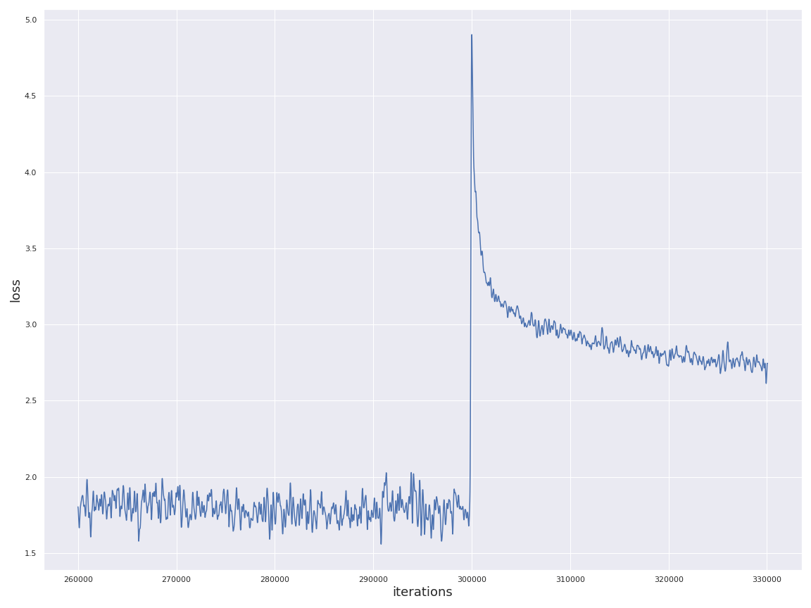
Noticeably, it’s picked up on certain highly-structured patterns, like the -nen and -sen endings common to Finnish and Norwegian surnames respectively. It’s also learned to generate significantly longer sequences, jumping from an average of 3.5 characters before producing the end-of-sequence mark to ~12 characters. That said, its training loss is significantly increased compared to that of the initial training stage – this is to be expected, both due to the shift in datasets between the initial training and the fine-tuning, and due to the increased entropy of character sequences fed from the name dataset compared to the more common words in Frankenstein.

We could, of course, let the model run for longer on the naming dataset, and probably reduce this loss a bit more. Realistically, this would likely cause it to start memorizing names from the relatively-limited inventory in Faker, so this is likely sufficient for our purposes.

Enforcer handles!

Finally, we’re ready (after saving another checkpoint for our model’s training state) for our final round, training directly on Enforcer handles. Since we’re dealing with a dataset orders of magnitude smaller than the general English text from the first round, it would be completely infeasible to train a model of this complexity directly on the Enforcer dataset. However, again, we’re able to leverage a lot of work on more general datasets to get our model most of the way there – ironically, brief training cycles on this data effectively causes it to unlearn some of its prior knowledge, though this suits our purposes in generating more interesting names!

After 20 epochs (necessary with our essentially toy-scale dataset) we can start sampling the network to generate names. Some favorites of mine (drawn from random one-to-three-character seeds):

seed --> output
---------------
a --> andelian
s --> saminthan
C --> Carili
b --> bestry
E --> EliTamit
G --> Gusty
L --> Landedbandareran
M --> Muldobban
I --> Imameson
T --> Thichy
G --> Gato
b --> boderton
K --> KardyBan
c --> cante
s --> sandestar
o --> oldarile
L --> Laulittyy
P --> Parielon
X --> Xilly
E --> Elburdelink
Be --> Beardog
Ew --> EwToon
Zz --> Zzandola
Ex --> Exi-Hard
Sp --> Spisfy
Sm --> Smandar
Yr --> Yrian
Fou --> Foush
Qwi --> Qwilly
Ixy --> IxyBardson
Abl --> Ablomalad
Ehn --> Ehnlach
Ooz --> Oozerntoon

Certainly silly, but any of these would be plausible as a handle, while being distinct from any of the input handles. The network has, to an extent, memorized patterns in existing Enforcer handles, so these do surface occasionally (particularly in evaluation mode, for the “most accurate” outputs), but any near-matches have been excluded here. I see this as an absolute win!

wrapping up

In this post, we saw how simple it is (on the order of 100 lines of straightforward, readable code) to lay out a performant recurrent neural network in PyTorch and use it to generate fun, fluid nicknames that’d fit in among any group of Enforcers. While we only had a relative handful of original handles to work with – far too few to train a model of this complexity – we were able to leverage other data sources (general English text, known personal names) to kickstart our learning process, enabling training on significantly smaller data with much faster iteration (running later training cycles in a reasonable timeframe even on CPU). While this transfer learning process is a powerful tool for training deep learning models, we must take a little care, as the further outside the original training domain our target data gets, the more we risk degraded performance.

We didn’t touch on a few more advanced topics, like using attention or variable teacher forcing during training (rather than the 100% forcing used here), or running our code on GPU. But we have seen that, using modern frameworks, it’s remarkably easy to build even a complex neural network! From a development standpoint, PyTorch’s long-standing emphasis on clean, Pythonic code made prototyping easy. Since PyTorch is designed to dynamically execute its graph, we can imperatively execute individual tensor operations on variable sequences, and examine our output in an interactive shell, which is fantastic for debugging (though Tensorflow 2.0 has introduced eager execution for its graphs as well).

All told, PyTorch probably has a shallower learning curve for a Python developer to start laying out functional code compared to Tensorflow, though there are still some design aspects (like the boilerplate needed to lay out a training loop) that I’m not too fond of. In any case, I’m excited to see a lot of the design decisions that I do like in PyTorch being brought into the Tensorflow ecosystem, while retaining its strengths (like the model-deployment story in tensorflow-serving).